Record a Macro in Excel

To automate the manual tasks you do repeatedly, you can use a simple macro. Below is an simple example of how we can use a macro to automate tasks

Consider for example a table of data as shown. And you need to repeatedly format a cell with a particular format (bold, bordered, background yellowed, font in red color).

Basic example of a macro

Step 1: Click the Record Macro button on the bottom left of excel window

Record button in Excel Window

Step 2: A dialogue box opens as shown below. Change the Macro name (if needed), put a shortcut key, scope of the macro and description. If you intend to use a lot of macros, it is a good practice to fill the details. Click Ok after all the details are filled.

Macro record dialogue box

Step 3: The macro continues recording until you manual stop the recording. Be careful what you do after the macro is recording. Do not change the selected cell. Change formatting of the cell (selected before recording a macro). Go to the Record Macro button (now the logo will be different and looks like a stop button) and click it. This stops the recording of the Macro.

Step 4: The macro is now ready to do manual tasks automatically. Select any cell and click the shortcut key chosen in Step 2. The cell will redo all the actions recorded by the macro.

Note: You will not be able to undo the changes you made using a Macro. Be careful with a Macro

Hope that helps,

Ramada

PS: please feel free to drop you excel/ word/ power point queries to mad.exceltips@gmail.com. I will try and respond as soon as I can. The more curious your question, the faster I respond.

Microsoft Word 'Document Map' Bug and work around

When I am working with a huge word document, I find using a 'Document Map' very convenient to navigate the whole document. However, there is one bug, which is persistent and annoying as hell. Thankfully there is a work around which I will explain in this post.

If you are unfamiliar with Document Map, please read my earlier post on Document Map (http://mad-exceltips.blogspot.com/2014/04/microsoft-word-document-map.html). 

With a document filled with content and Document Map enabled, originally looks like this

Document Map in Microsoft Word

However, when you close and open the document, the Document Map jumbles up as below. 

Jumbled Document Map after re-opening the document

Before knowing the workaround, I have reorganized the Document Map numerous times, before I got annoyed and looked for a workaround. The work around doesn't really fix the bug, but if you follow few practices, the Document Map will remain the same. 

The issues is, Word re-formats the document when you re-open the document. Keep an eye on the bottom right (left of zoom options), when you open the document. First, Word says 'Opening' then jumps to 'Word is formatting the document'. If it says, 'Word is formatting the document' that is when the bug is introduced. And after the document is opened, the Document Map will look all jumbled up.

The workaround is

1. The moment, you see 'Word is formatting the document'; do not save the document. If you save it, the new format will be saved. 
2. Instead, go to View -> Un-check Document Map
3. Close the document without saving it.
4. Re-open the document. Now, it shouldn't say 'Word is formatting the document'. If it still does, do mail me. We will figure out a workaround.
5. After you open the document, go to View -> Check Document Map. Bingo !! The map is intact. 

Any deviations, from what I described above; or better workarounds, please do mail me. Would be happy to listen.

Hope that helps,

Ramada

PS: please feel free to drop you excel/ word/ power point queries to mad.exceltips@gmail.com. I will try and respond as soon as I can. The more curious your question, the faster I respond.

Bubble Chart with Text inside the bubble

Bubble chart is a concise and crisp way of presenting data with 3 dimensions. However the main challenge of creating a bubble chart is; 'to have the text (names/ regions/ countries/ products) within the bubble'

Assuming we have 4 people data of Age, Weight and Height. The data is as below

	Age	Weight	Height
John	28	70	7
Michael	50	34	6
Vicky	34	60	8
Neil	15	27	10

If we create a bubble chart by selecting this data we get something like below

Basic bubble chart with data labels

It is very difficult to determine which bubble belongs to which person. And to enter the persons name into the bubble charts, there is no automatic way in excel. Depending on the number of rows, this task can be very tedious and time consuming.

Thankfully, the bubble chart VBA code (provided at the end) can do this in a click. Follow the below steps

1. Open a new excel workbook, 
2. Press Alt F11. This takes you to Microsoft Visual Basic Editor
3. Copy the below VBA code from "Public Sub... End Sub" and paste it into the above opened window
4. Close the VBA editor.
5. In the workbook, go to Insert -> Shapes -> Select a Rectangle. Draw a rectangle on your sheet. 
6. Right click the rectangle, and click Assign Macro. From the list, select a row which ends with CreateBubbleChart2. This makes the rectangle shape a button. Try clicking it. It should say 'Selection must have 4 columns and at least 2 rows'. If you see this message, Bingo !! its working. 
7. To test this, copy paste the table provided above. Select the data (4 columns and 5 rows) and click the rectangle. This should create a bubble chart as below in a new sheet.
8. When you close, make sure you Save As 'Excel Macro-Enabled Workbook' (this selection can be found just below the space where you enter file name. 

Bubble chart created using the VBA code below

Hope this helps.
-Ramada

PS: please feel free to drop you excel/ word/ power point queries to mad.exceltips@gmail.com. I will try and respond as soon as I can. The more curious your question, the faster I respond.

Public Sub CreateBubbleChart2()

    If (Selection.Columns.Count <> 4 Or Selection.Rows.Count < 3) Then
        MsgBox "Selection must have 4 columns and at least 2 rows"
        Exit Sub
    End If

    Dim SelectedRange As Range
    Set SelectedRange = Selection

    Sheets.Add After:=Sheets(Sheets.Count)

    Dim bubbleChart As ChartObject
    Set bubbleChart = ActiveSheet.ChartObjects.Add(Left:=1, Width:=600, Top:=1, Height:=400)
    bubbleChart.Chart.ChartType = xlBubble
    Dim r As Integer
    For r = 2 To SelectedRange.Rows.Count
        With bubbleChart.Chart.SeriesCollection.NewSeries
            .Name = "=" & SelectedRange.Cells(r, 1).Address(External:=True)
            .XValues = SelectedRange.Cells(r, 2).Address(External:=True)
            .Values = SelectedRange.Cells(r, 3).Address(External:=True)
            .BubbleSizes = SelectedRange.Cells(r, 4).Address(External:=True)
        End With

    Next

    bubbleChart.Chart.SetElement (msoElementPrimaryCategoryAxisTitleAdjacentToAxis)
    bubbleChart.Chart.Axes(xlCategory, xlPrimary).AxisTitle.Text = "=" & SelectedRange.Cells(1, 2).Address(External:=True)

    bubbleChart.Chart.SetElement (msoElementPrimaryValueAxisTitleRotated)
    bubbleChart.Chart.Axes(xlValue, xlPrimary).AxisTitle.Text = "=" & SelectedRange.Cells(1, 3).Address(External:=True)

    bubbleChart.Chart.SetElement (msoElementPrimaryCategoryGridLinesMajor)
    bubbleChart.Chart.Axes(xlCategory).MinimumScale = 0

    ActiveSheet.ChartObjects(1).Activate
    Dim srs As Series
    For Each srs In ActiveChart.SeriesCollection
        srs.ApplyDataLabels AutoText:=True, LegendKey:=False, _
            ShowSeriesName:=True, ShowCategoryName:=False, ShowValue:=False, _
            ShowPercentage:=False, ShowBubbleSize:=False
        srs.DataLabels.Position = xlLabelPositionCenter
    Next srs

    ActiveChart.SetElement (msoElementLegendNone)

End Sub

Microsoft Word Document Map

When I am working with a huge word document, I find using a 'Document Map' very convenient to navigate the whole document.

Go to Microsoft Word -> View -> Second section has 'Document Map'.

Document Map with Default 'Thumbnails' as checked

A new document generally opens with Thumbnails checked. The below is an example of a Thumbnail for a document with content. With Thumbnails it is generally very difficult to navigate a document with more than 30 pages.

Thumbnails in Microsoft Word

If you click 'Document Map', 'Thumbnails' Automatically goes unchecked. The document with above 'Thumbnail' looks like below with a Document Map. It looks more organized, easier to jump sections, see the story line of the document. It is similar to Table of Contents, but available all the time. 

Document Map in Microsoft Word

Note that Document Map works similar to Automated Table of Contents. It uses the Heading formatting to populate the document map.

Hope that helps,
Ramada

PS: please feel free to drop you excel/ word/ power point queries to mad.exceltips@gmail.com. I will try and respond as soon as I can. The more curious your question, the faster I respond.

Excel business usage and context

We generally start using excel without really knowing how it revolutionized 'analysis'. In practical terms, it doesn't matter whether you know its history or not. However, with some knowledge, you can understand the power of the tool and why it is so prevalent in the current business environment. It is one tool which is the most underrated but mastering it can save a lot of time. Thanks to my B-school, I learnt very advanced usage of excel without realizing its necessity in the context.

Excel has existed in some form since 1961 and has its roots in practices used for ledger keeping. The excel in the current context is mainly used for 'data storage, table based, quick analysis' with limited data.

When I was younger, my school used to keep a record for attendance like the one below

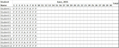
A general ledger for Student attendance in schools

The teacher populated this ledger everyday and at the end of the month provides a summary information to parents and also the school management. With excel, the preparation of summary report including total number of days present, % of attendance, specific day attendance is done within few minutes. There is also benefit in formatting to make the sheets look more effective.

The above example is the most basic function of excel.

The school management used to post a customized attendance letter/ SMS to each parent with their kids performance. The students attendance is in one table, and the students address, parents name, parents phone number is in another table. In a manual scenario, the teacher will have to look for address of each student, draft a letter with his performance and post it. This is again a tedious and error prone process. With excel, the table with attendance performance and table with personal details can be linked with basic formulae like VLOOKUP. The job can be done in 5-10 minutes.

In my view, 40%-50% people using excel, would use it for a business context similar to above.

The advanced excel users are typically consultants, analysts and investment bankers who run scenarios, financial modeling, financial estimations etc.

There is pretty much nothing, that you cannot do with excel and the associated VBA (this is the programming language that excel runs on). But the complicated the analysis, the bigger the data, the importance of data security will change the tool that you are going to use. For ad-hoc analysis (which is almost 60%-70% of employee usage), excel works fine.

PS: PS: please feel free to drop you excel/ word/ power point queries to mad.exceltips@gmail.com. I will try and respond as soon as I can. The more curious your question, the faster I respond.

Frequently used Excel Shortcuts

Some of the frequently used shortcuts of Excel are (highly useful shortcuts in my view are highlighted)

WORKING WITH WORKSHEETS
Move to the next sheet in the workbook	CTRL+PAGE DOWN
Move to the previous sheet in the workbook	CTRL+PAGE UP
DATA ENTRY
Start a new line in the same cell	ALT+ENTER
Insert a hyperlink	CTRL+K
Insert a comment	SHIFT+F2
Repeat the last action	F4
MOVE AND SCROLL WITHIN WORKSHEETS
Move to the beginning of the worksheet	CTRL+HOME
Move to the last cell on the worksheet, in the bottom-most used row of the rightmost used column	CTRL+END
Move one screen to the right	ALT+PAGE DOWN
Move one screen to the left	ALT+PAGE UP
FORMATTING
Apply the General number format	CTRL+SHIFT+~
Apply the Number format with two decimal places, thousands separator, and minus sign (–) for negative values	CTRL+SHIFT+!
Apply the Currency format with two decimal places (negative numbers in parentheses)	CTRL+SHIFT+$
Apply the Percentage format with no decimal places	CTRL+SHIFT+%
Apply the outline border to the selected cells	CTRL+SHIFT+&
Remove the outline border from the selected cells	CTRL+SHIFT+_
BORDERING - in the FORMAT CELLS dialog box (CTRL+1)
Apply or remove the top border	ALT+T
Apply or remove the bottom border	ALT+B
Apply or remove the left border	ALT+L
Apply or remove the right border	ALT+R
If cells in multiple rows are selected, apply or remove the horizontal divider	ALT+H
If cells in multiple columns are selected, apply or remove the vertical divider	ALT+V
Apply or remove the downward diagonal border	ALT+D
Apply or remove the upward diagonal border	ALT+U

PS: please feel free to drop you excel/ word/ power point queries to mad.exceltips@gmail.com. I will try and respond as soon as I can. The more curious your question, the faster I respond.